Weekly Chart Review

Quarterly Update: Average Investor Allocation to Equities Model

Hey everyone, it’s Jim.

Hope you had a great weekend—and to all the Dads out there, Happy Father’s Day!

Let’s jump into this week’s newsletter. We’ve got a big one, including our latest quarterly update to the Average Investor Allocation to Equities model and much more!

---

In this week’s newsletter:

• Stay Informed

  • Key Macro Events From Last Week (ICYMI)

  • Key Macro Events To Watch This Week

• The Market Map

  • Application - S&P 500

• Deep Dive

  • Quarterly Update: Average Investor Allocation to Equities Model

• S&P 500 Fair Value Model

• The Market Map - Extended Analysis

  • Major US Indices

  • 11 Major US Equity Sectors

  • US Treasuries

---

Stay Informed

Key Macro Events From Last Week (ICYMI)

Here’s what moved markets last week:

📊 Consumer Price Index (CPI – May)

• CPI (MoM): Rose 0.1% in May, down from April’s 0.2% increase.

• CPI (YoY): Increased 2.4%, up from 2.3% in April.

• Core CPI (MoM): Excluding food and energy, up 0.1% (vs. +0.3% expected).

• Core CPI (YoY): Unchanged at 2.8%. (Link)

---

🏭 Producer Price Index (PPI – May)

• PPI (MoM): Final demand rose 0.1%, rebounding after April’s –0.2%.

• PPI (YoY): Increased 2.6% over the past 12 months.

• Core PPI (MoM): Core (ex-food, energy, trade services) also rose 0.1%.

• Core PPI (YoY): Registered a 2.7% annual increase. (Link)

---

🧾 Jobless Claims (week ending June 7)

• Initial claims: Held at 248,000, the highest level in eight months.

• Continuing claims: Increased to approximately 1.95 million, the highest since November 2021. (Link)

---

🔍 Broader Economic Context

• Inflation outlook: May’s inflation data shows cooling price pressures, though some risk remains from tariff-driven goods prices.

• Fed expectations: Data bolsters expectations of the Federal Reserve starting rate cuts in September 2025, though June’s meeting will likely maintain current rates at 4.25%–4.50%.

• Labor market: Rising jobless claims hint at a slowing labor market, yet no immediate signs of recession.

---

Key Macro Events To Watch This Week

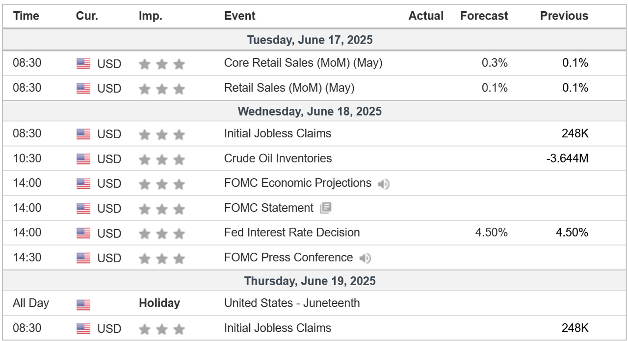
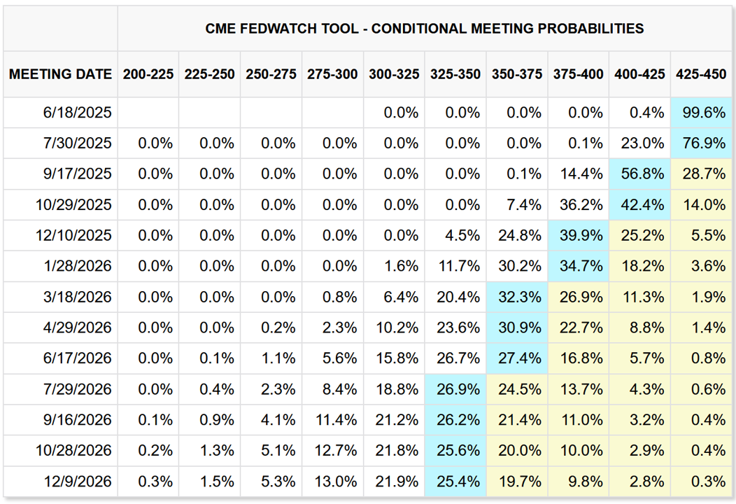
The key economic event this week will be the FOMC rate decision on Wednesday.

Fed Funds futures currently suggest there is a 99.6% probability that the Fed will leave rates unchanged at 4.25% - 4.50%.

Further, the market is suggesting that the first rate cut will not occur until the September meeting.

Go here if you want to monitor the Fed Funds futures in real-time.

---

Paid subscribers get access to our proprietary S&P 500 Fair Value Model, tactical sector signals, and timing tools—see below for how this can help in the current market environment.

🟢 Special Offer: Get lifetime access to institutional-grade models for less than $10/month (normally $33)—only available to the next 10 subscribers.

---

The Market Map - Application - S&P 500

The S&P 500 returned -0.39% last week and remains in a technical downtrend according to our analysis.

Through Thursday, the S&P 500 was better by 0.75%, but Friday’s decline of -1.13%, on the back of the Israel/Iran conflict, is what put us in negative territory.

With that said, we’ve had a few key developments this week on the technical front.

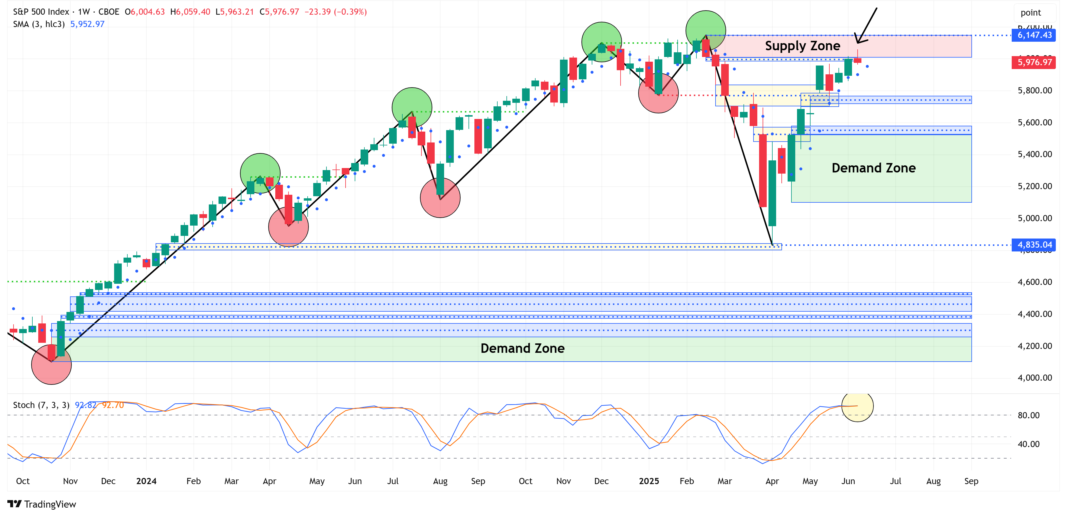
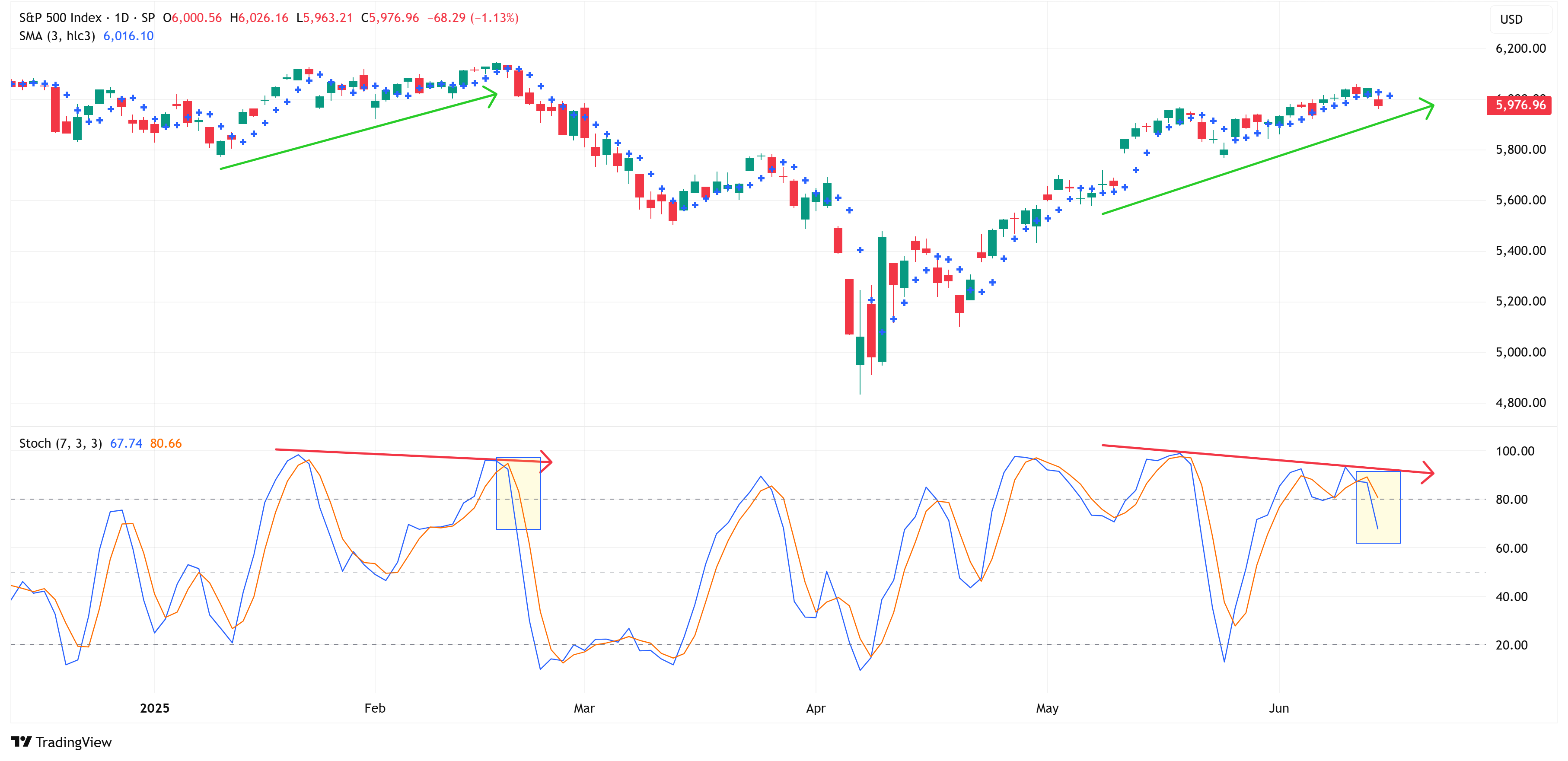
Let’s start with the weekly chart that we have focused on for several months now.

Today, I’m going to introduce “supply zones” and “demand zones”.

Very simply, supply zones are typically areas where one would want to sell from, while demand zones are areas where one would want to buy from.

The S&P 500 “wicked” into a supply zone last week (see black arrow), which suggests that this supply zone has now been mitigated, and the market could theoretically head lower from here.

Also, note that our stochastic indicator continues to remain overbought (yellow circle in bottom panel), further suggesting that buying momentum could be slowing.

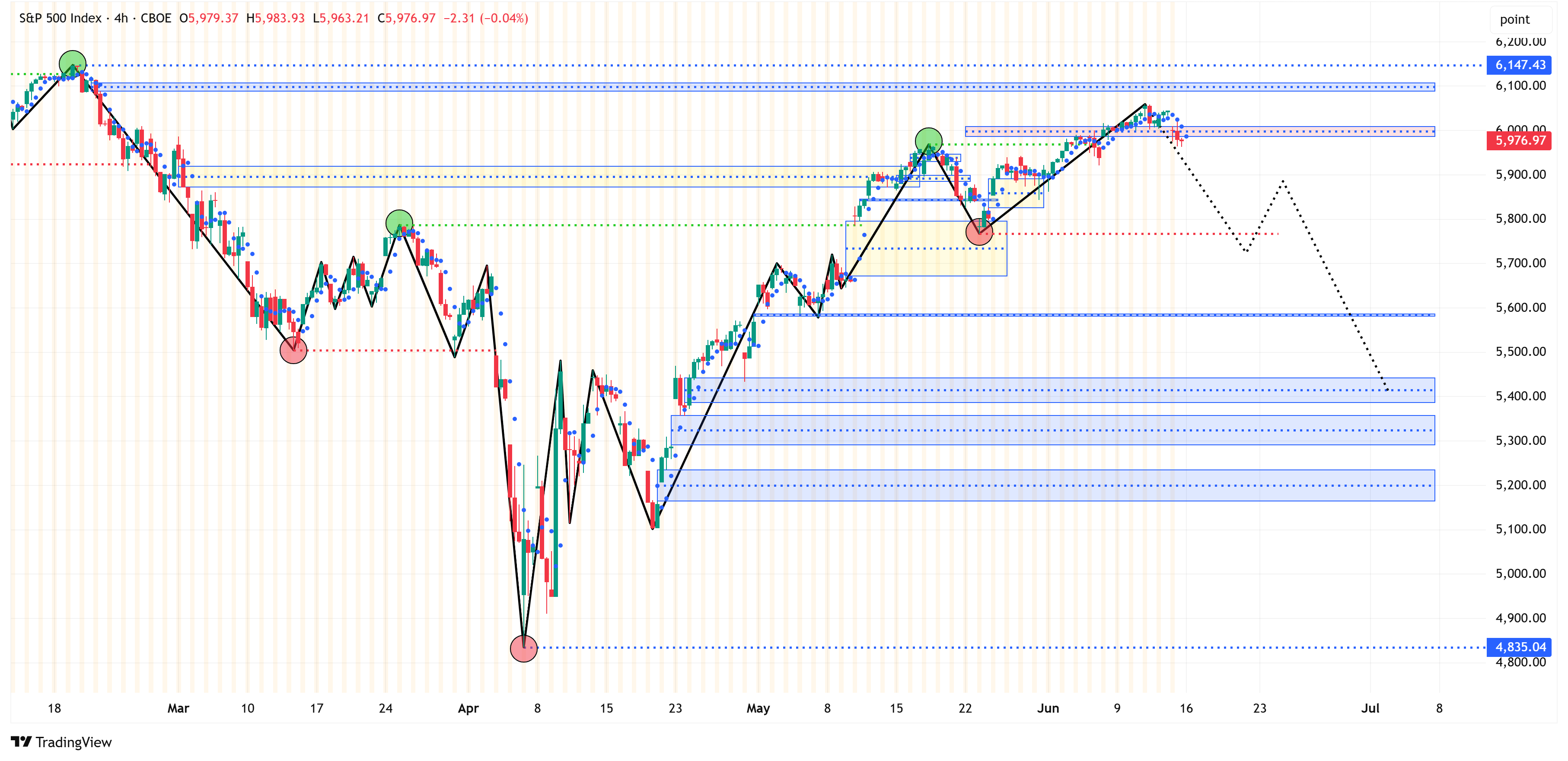
Now, let’s shift to our 4-hour time frame to see if it gives us any additional clues.

The 4-hour time frame remains bullish but has started to turn lower.

In the current setup, the 4-hour time frame would have to fall below the horizontal red line that I’ve drawn to officially turn bearish.

The black dotted line is one possible path the S&P 500 could take on the 4-hour time frame.

Lastly, I want to look at the S&P 500 on the daily chart and specifically, I want to draw your attention to the negative divergence that has developed, which is very similar to what we saw happen earlier in the year.

For those not familiar with negative divergences, here’s a quick primer:

In technical analysis, a negative divergence occurs when the price of an asset makes a higher high, but a technical indicator (such as RSI, MACD, stochastic oscillator, or volume) makes a lower high. This divergence suggests that momentum is weakening, even though prices are still rising.

🔍 What it means:

• It’s often interpreted as a bearish signal, indicating that the current uptrend may be losing strength and a potential reversal or correction could be ahead.

• Traders use it to anticipate a shift in trend, especially when it appears after a prolonged uptrend.

✅ Example:

• The S&P 500 makes a new high, but the stochastic oscillator forms a lower high.

• This could signal that fewer stocks are participating in the rally or that buying pressure is fading.

📉 Common indicators used for spotting negative divergence:

• Relative Strength Index (RSI)

• Moving Average Convergence Divergence (MACD)

• Stochastic Oscillator

• On-Balance Volume (OBV)

In summary, our analysis of the S&P 500 suggests that the chances of a downturn are increasing, as we have multiple confluences of evidence suggesting a similar short-to-medium term narrative.

---

If you’re finding this helpful, consider sharing it with a colleague. It helps us grow and lets us keep providing this research each week.

---

Deep Dive

Quarterly Update: Average Investor Allocation to Equities Model…

Let’s start with the chart and then get into the analysis and takeaways.

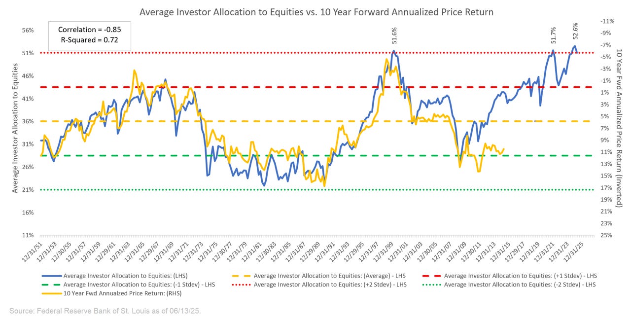
For those who may be new to our newsletter and this model, here is how to read the chart above:

“The blue line in the chart shows the “Average Investor Allocation to Equities”. As the name would imply, this line shows how much (i.e., what percentage) of the average investor’s portfolio is allocated to equities at any given time as opposed to other asset classes (i.e., fixed income, commodities, cash, etc.) This line maps to the left-hand scale of the chart.

The yellow line in the chart shows the “10-Year Forward Annualized Price Return” of the S&P 500 Index. This tells us what the 10-year forward return was for the S&P 500 Index from the corresponding point on the blue line. This line maps to the right-hand scale of the chart and the values have been inverted to better show the relationship between the two metrics.”

Next, we want to understand how to interpret this chart:

“Very simply, the higher the blue line (i.e., the “Average Investor Allocation to Equities”), the lower the subsequent 10-year return for the S&P 500 Index and vice versa.”

---

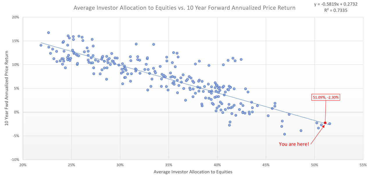
In the chart below, the blue dots represent actual historical data.

• X-Axis = Actual historical “Average Investor Allocation to Equities” values.

• Y-Axis = Actual historical “10 Year Fwd Annualized Price Return” values.

Note the “You are here!” value (red dot).

This marks our most recent model value of 51.1%, which we then combine with a regression-based model output of -2.30% for the 10-Year Fwd Annualized Price Return of the S&P 500.

This means that over the next 10 years (March 31, 2025, to March 31, 2035), our model suggests that the S&P 500 will have an annualized return of -2.30%.

---

The following chart is the same as the first one above, but I’ve broken it down into three different segments.

The first two segments represent a full cycle (i.e., trough-peak-trough) for the Average Investor Allocation to Equities.

The third segment is the current cycle, which is not yet completed.

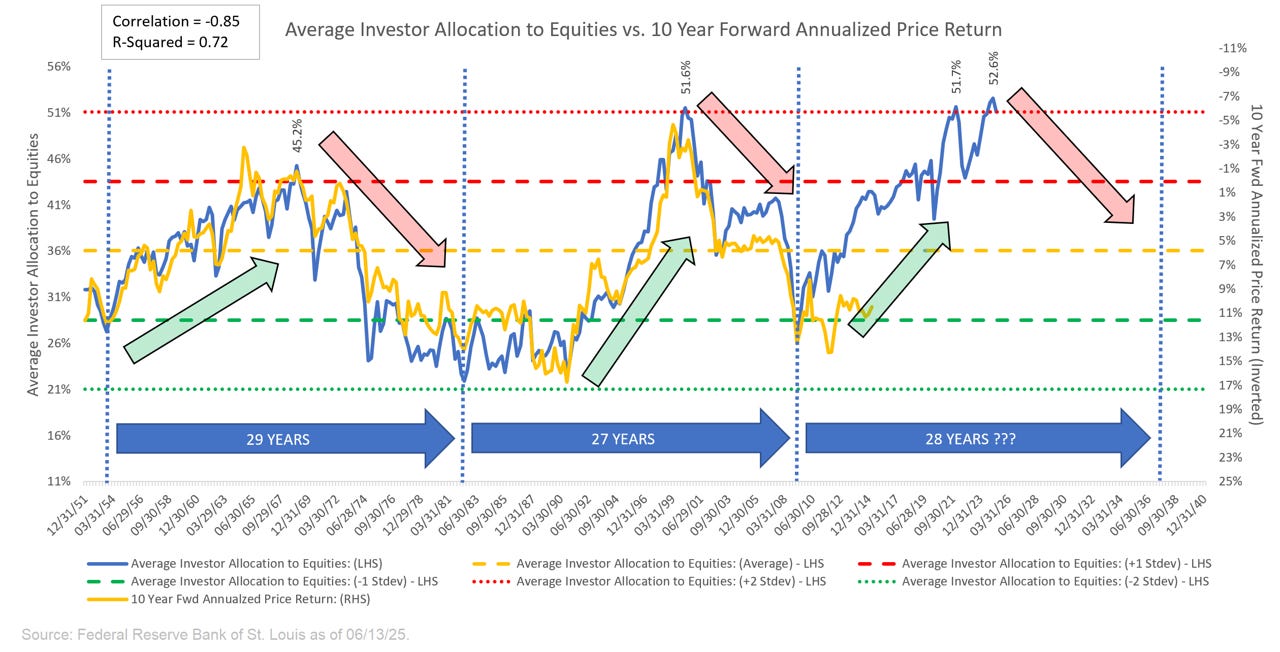
Note in the chart above that I have used green/red arrows to denote up/down trends for the Average Investor Allocation to Equities.

Here is what those same periods (green/red arrows) look like when we chart the S&P 500. Note: the grey vertical bars represent US recessions.

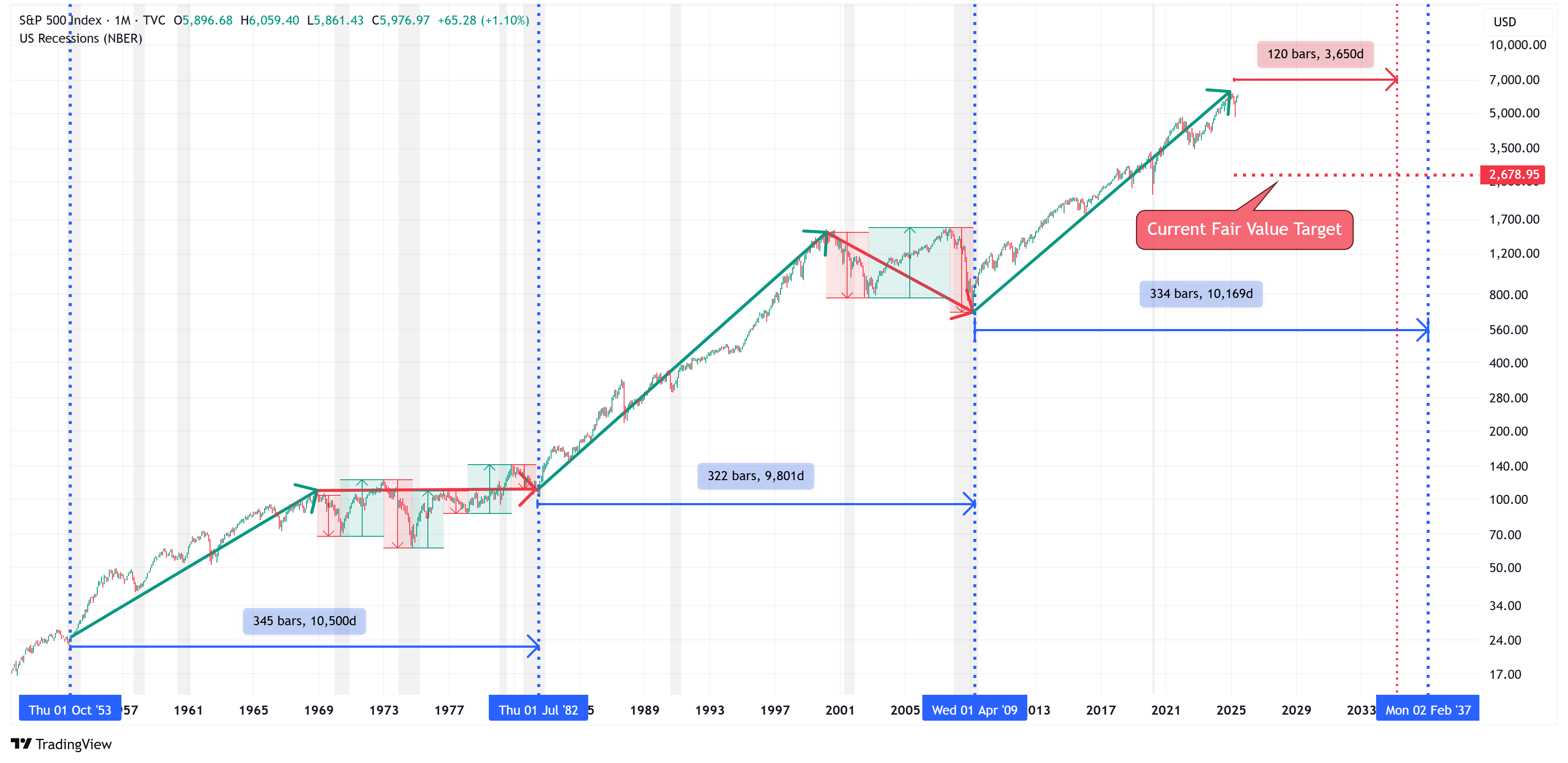
In addition to the green/red arrows noted above, I have added blue vertical lines to denote the start/end of the three cycles.

Further, I have drawn a red vertical line to denote the end of the 10-year period referenced above (March 31, 2025, to March 31, 2035).

This 10-year period, and the end of the proposed third cycle (February 2037), are not far apart, especially when we consider that I’m using an average of the first and second cycles to come up with a period of 334 months for the third cycle. Could the third cycle be as short (or shorter) as the second cycle (322 months)? Anything is possible.

Net/net, the model is suggesting an end to this current cycle somewhere in the context of 2035-2037 (give or take a year or two).

Lastly, I have inserted a horizontal red line to depict the current fair value (2,678.95) from our Average Investor Allocation to Equities model.

Note: On July 1st, the fair value for the Average Investor Allocation to Equities model will move to 2,752.34 or 2.7% higher than the current value.

---

Putting it all together…

Unless we see a significant change (and soon) in the global financial picture, the next 10 years will likely be different and potentially more volatile than the previous 10 years.

This is not a doom-and-gloom forecast; instead, it’s a call to encourage our readers to think differently about asset allocation over the next 10 years, as I believe many new and different opportunities will present themselves.

What has worked well over the last 10 years may not work as well over the next 10 years, and vice versa.

With that said, look at the end of the last two cycles in the charts above and think about how your portfolio would have performed had you been overweight equities at the end of the previous two cycles. It’s not time to do that, but you want to have dry powder when that opportunity presents itself.

One of the benefits of our S&P 500 Fair Value Model (which paid subscribers receive each week) is that it gives us a very good indication of when the bottom may be in.

This creates a signal giving us a high probability time to get overweight equities, and conversely, a signal for when to remove some of the more protective measures we may have deployed leading up to that point.

If you would like access to our proprietary indicators, consider becoming a paid subscriber.

---

The sections that follow are for paid subscribers only.

In these sections, we will discuss our proprietary:

• S&P 500 Fair Value Model

  • This model provides a guide for a) how far the S&P 500 could decline in the next recession and b) when to get back into the market after it has declined.

• “The Market Map” - Systematic Process

  • We will call out specific price objectives (up trends vs. down trends, targets, stop losses, etc.) on the following:

    • Major US Indices

    • 11 Major US Equity Sectors

    • US Treasuries

🟢 Special Offer: Get lifetime access to institutional-grade models for less than $10/month (normally $33)—only available to the next 10 subscribers.